1-2: Math Mode
In the previous lessons you created some simple LaTeX documents. This lesson is the first one where you will put mathematics into your document.
It’s all about the $dollar signs$
To tell LaTeX that you want to typeset mathematics, you surround math markup commands with single dollar signs. Here’s an example of a complete document, using the same framework as before, that introduces a little bit of mathematics.
\documentclass{article}
\begin{document}
The Pythagorean Theorem is that in a right-angled triangle, the equality $a^2+b^2=c^2$ always holds, where $c$ is the length of the hypotenuse and $a$ and $b$ are the lengths of the legs.
\end{document}
Try compiling this document. When you succeed, you’ll get a one-page .pdf document which looks like this:

Pretty excellent! Now let’s look at the source code. There were four different math sections contained in dollar signs: one with the formula, and three containing just the variable names. Notice that in math mode all variable names are displayed in italics by default; this is a convention followed by all mathematicians and helps distinguish variables from normal text.
The only complicated expression inside of dollar signs is $a^2+b^2=c^2$. The caret sign (^) is used in LaTeX to designate an exponent. As you can see, LaTeX will typeset the exponent like a superscript: it doesn’t show ^, but instead the exponent is raised and showed in a smaller font.
Adding extra space inside of math mode expressions is optional and has no effect: you’ll get exactly the same result if you change the input to $a^2 +b^2= c^2$. Try this yourself!
We’re going to continue with some additional examples below. We’re not going to repeat the boilerplate stuff every time; instead, use this template to compile each example.
\documentclass{article}
\begin{document}
% put the stuff you want to typeset here
\end{document}
Nesting
Working with more complicated exponents is a good example of how nesting works in math markup. This is a pretty logical looking piece of text:
The number starting with 1 and followed by 100 zeroes is called a googol. Written using exponents, a googol is equal to $10^100$.
However, when you typeset it, the number at the very end will look wrong, like this:

This is a problem: we wanted the exponent to be 100, but instead LaTeX only put 1 as the exponent, and did not include the 00. The reason for this problem is that in general, LaTeX will assume that an operator like ^ will only apply to a single character; you can override this by explicitly wrapping the whole target expression in curly braces {}. So by changing our LaTeX code to
$10^{100}$
we get the correct result:
![]()
Try it for yourself!
LaTeX is very flexible. You can put anything that you like as the base or the exponent, including another exponential. For example, if you write
$10^{10^{2}}$
then this will create a nested exponent!

This is a concrete example of why using LaTeX is a lot nicer than a wysiwyg editor such as Microsoft Word: creating multiple levels of subscripts in different sizes and at different heights is handled automatically for you.
Exercise (nickname: exponents)
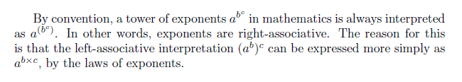
To get the part 
b \times c.
Subscripts
Subscripts are very similar to exponents/superscripts. Whereas you use ^ for superscripts, you use the underline character _ for subscripts. For example, writing
Eight, in binary, looks like a thousand: $8 = 1000_2$.
gives you

LaTeX is smart when it comes to combining subscripts and superscripts. Writing a^b_c or a_c^b gives you

Remember to use {} to contain long subscripts just like you would with superscripts.
$$Display mode$$ and sums
Writing summations like

is also done with the subscript and superscript operators:
\sum_{i=1}^n 2i-1
However if you try this using the previous template, you’ll get something slightly different that looks like 
As you may have already noticed, the way that the course nodes are laid out, sometimes we put mathematical LaTeX inside the middle of a paragraph like this 

The first kind of typesetting is called inline and the second kind is called display typesetting. As a rule of thumb, inline typesetting is used to cause minimal disturbance to the flow of the text, while display is used to explicitly emphasize and distinguish a piece of text from its surroundings. (It’s not limited to math, for example these notes use multiple styles of source code too.)
Whereas LaTeX uses $single dollar signs$ to contain inline math, it uses $$double dollar signs$$ to contain display math. Here’s an example showing both kinds of displays: the source code
Inline looks like $\sum_{i=1}^n 2i-1$, while display looks like $$\sum_{i=1}^n 2i-1.$$
gives

As a side effect, you can see that the sums are typeset somewhat differently in the two modes. In inline, the parts n and i=1 of the sum are squished to the side, in order to avoid the line of text from getting too tall. In display, you get the correct version of the typesetting, where the bounds really appear below and above the summation symbol. When you have a long or complex formula, try both modes, and you may notice that it looks better in display mode, and has more whitespace to make the presentation look more pleasing.
There are other symbols like \sum: for example \prod for product, \int for integral, \lim for limit, and \mathop to define new ones.
Exercise (nickname: limit)

You will need to use t \to \infty as a subscript on \lim in order to get 
Roots and Fractions
To conclude the lesson, we give two more useful constructions. To typeset the square root symbol, use \sqrt{} with the desired content of the square root inside of the curly brackets:
\sqrt{4}=2 gives 
If you want a cube root or any other kind of root, use
\sqrt[a]{b} to obtain ![\sqrt[a]{b}](http://s.wordpress.com/latex.php?latex=%5Csqrt%5Ba%5D%7Bb%7D&bg=ffffff&fg=000000&s=0 "\sqrt[a]{b}")
You use square brackets here because that is the way that LaTeX indicates an optional argument.
You can use / as a normal division symbol, like a/b giving \(a/b\), but to get a fraction where the numerator and denominator are above and below a horizontal line, use the \frac{}{} command. It takes two arguments, the first one being the numerator and the second one the denominator. It will be typeset slightly differently depending on whether your mode is inline or display:
Inline looks like $\frac{1}{2}=0.5,
nbsp;while display looks like $\frac{1}{2}=0.5.$
gives

There are commands dfrac and tfrac to override which style is used, but we won’t talk about them since the default style will be fine for our purposes.
Exercise (nickname: fractions)

Use \cdots to get the centred ellipsis \(\cdots\) symbol. We’ll take about the ellipsis more later…
If you need inline math to appear as it does in display mode, you can use the \displaystyle command to do so. For example,
Inline with \textbackslash displaystyle looks like $\displaystyle\frac{1}{2}=0.5$.
gives \[\textrm{Inline with \displaystyle looks like }\frac{1}{2}=0.5.\] This fuction may be useful for a one-line question on a math test, but be cautious using this in a multi-line paragraph, as the distance between lines may need to be adjusted to fit the math in.