M-3: Plots, Functions, Sets, Lists, and Sequences

Maple is able to plot functions in a variety of formats. We’re going to start with the simplest usage,

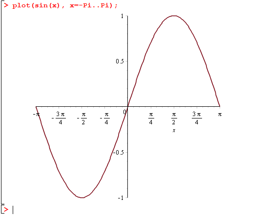
> plot(sin(x), x=-Pi..Pi);

which will give you something that looks like this:

In this case, we explicitly specified the x-range, and Maple chose the y-range automatically based on the minimum and maximum values. Notice that by right-clicking (PC) or command-clicking (Mac) on the plot, you will see a number of options, including an Export option which includes the .eps format. (This may be useful for your final project! You can export to .pdf too but it has far too much whitespace. To get around this, either use the trim option of includegraphics, or export to .eps and convert from eps to pdf if necessary.)

You will also see some different options about colour, style, axes, scaling, etc. However, we’re only going to focus on the command-line versions of these options, since they are more consistently reproducible; as far as we know every option can be specified textually. For example, let’s say that we don’t like how the picture is stretched out of proportion. We can send plot() an explicit y-range of -3..3 by typing

> plot(sin(x), x=-Pi..Pi, -3..3);

and you will see that this looks a bit better. However, many people would prefer

> plot(sin(x), x=-Pi..Pi, scaling=constrained);

which has a y-axis of the right length too. Like many other Maple functions, plot is very versatile and accepts many different types of inputs and named arguments. On the help pages ?plot, ?plot/details and ?plot/options you can see some of them. (Caveat: we’ll discuss {sets} and [lists] below, which are needed to understand some of the options.)

In the example above we used the format  plot(expr, x=a..b, opts) where scaling was the only option we chose to specify. Setting a second option is done just by appending to the end of the plot call,

> plot(sin(x), x=-Pi..Pi, scaling=constrained, legend=["Sine function"]);

Try this and see what it gives you.  Note: we’re using "double quotes" here to define a String/text chunk literal, while we introduced the 'single quote' in the previous lesson (just before introducing restart) which does delayed evaluation (see ?'). Finally `back-quotes` are used to write symbol literals (but we have some feedback from students saying this does not work on a Mac).

Functions

How can we define a new mathematical function in Maple? Let’s try to define a function to compute the square of a number. The first thing you might try is

> square(x) := x^2;

and while this seems ok, the result is not effective: square(4) does not work if you try it on the next line. (What you’ve done is hard-code a single input/output pair, so calling square(x) works, but square(y) doesn’t.) The correct way to define this sort of function is the following:

> square := x -> x^2;

Try it and confirm that square(4) works on the next line. Note: the motivation for this notation is that we want to redefine square to mean “the function which maps any \(x\) to \(x^2\).” The mathematical notation for such a function is \(x \mapsto x^2\) (\mapsto in LaTeX), and Maple’s mimicing that concept.

In the above definition, we’re adhering very closely to the mathematical definition of a function: a map that specifies, for every input, a single output value. Consequently, when we use square with plot, it is no longer necessary to refer to the variable name x: try it for yourself by running the command

 > plot(square, -4..4);

Verify that it is a plot of the square function over the domain [-4, 4].

Just like in mathematics, Maple can define a function that takes in more than one argument. This is done using the syntax

> «function name» := («arg1», «arg2») -> «function definition»;

(Three or more arguments are also possible.) For example,

> gaussian2D := (x, y) -> exp(-x^2-y^2)/Pi;

will define a function representing the probability density of the standard bivariate Gaussian. Check that it works:

> gaussian2D(1, 1/2);        # gives exp(-5/4)/Pi
> evalf(gaussian2D(1, 1/2)); # gives 0.091197...

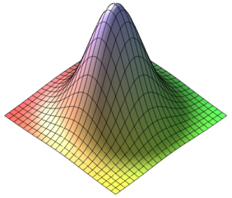
Let’s return to the gaussian2D example: we can even plot it as a 3-D graph. This is done with the plot3d command. Type in either one of the following commands:

> plot3d(gaussian2D, -2..2, -2..2);
> plot3d(gaussian2D(a, b), a=-2..2, b=-2..2);

and you’ll get a picture like the following:

Right-click on it to access the style options, and in particular choose the Manipulator drop-down menu and select Rotate. This will let you interactively rotate the plot by clicking on it and dragging your mouse in different directions.

Sets and Lists

Sets and lists are the two fundamental structured data types in Maple. Here are two examples:

> mySet := {1, 2, 3};
> myList := [1, 2, 3];

What is the difference between a set and a list? The difference, like in mathematics, is that a set has no inherent order on its elements and does not allow repeats, while order and repetition are important for lists. (Sometimes you might mathematically say tuple instead of a list.) We can verify this as follows:

> evalb({1, 2, 3} = {3, 1, 2, 1});  # true
> evalb([1, 2, 3] = [3, 2, 1]);     # false

One place where you’ll need to use a list is if you want to plot multiple functions on the same set of axes. Try

> plot([sin(x), cos(x)], x=-Pi..Pi, legend=["Sine", "Cosine"]);

Here is a question worth understanding: why do we logically have to use a list here, and not a set?

An example application of sets is to use as an argument to solve, when we want to solve multiple equations for multiple unknowns. Try

> solve({x+y = 1, 2*x - 3*y = 4}, {x, y});

Here, solve would also be happy to accept a list… often you can use either unless one is logically required.

More about sets

You can take the intersection, union, and difference of sets using the Maple operators named intersect, union, and minus.

> ({1, 2, 3} union {2, 3, 4}) minus {2}; # gives {1, 3, 4}

More about lists

Once you have a list, you can access individual elements using indices: [1] refers to the first item, [2] is the second, etc.

> names := ["alice", "bob", "carl", "doris"];
> names[2];                           # gives "bob"
> names[2] := "robert";               # change 2nd value
> names;                              # ["alice, "robert", "carl", "doris"]

Caveat: you can only set someList[i] to a value when someList already exists and has length at least i. This generally means that in order to use lists as data structures, you must explicitly initialize them, e.g. with someList := [seq(0, i=1..desiredLength)]. For advanced usage we’d use Arrays — they won’t be covered in detail but we’ll mention them again at the end of the case study in lesson M-7.

Gluing lists and converting sets/lists with op

Occasionally you may want to convert a set to a list or vice-versa. One way to accomplish this is with the op() function, which strips a list or set of its parentheses. Say that we’ve defined names as above; then

 > op(names);

will give back the comma-delimited sequence

“alice”, “bob”, “carl”, “doris”

without any surrounding brackets or braces. This is an expression sequence. Wrapping an expression sequence in {} turns it in to a set, and wrapping it in [] turns it in to a list, and in this way you can convert sets to lists and vice-versa. Furthermore, you can concatenate two expression sequences using commas: for example,

> [op(names), "ed", "fritz"];

will give back the list

[“alice”, “bob”, “carl”, “doris”, “ed”, “fritz”]

Small print: op() has other purposes too, such as extracting parts of a Maple expression, but we leave this out of our lessons. See ?op for the details.

Creating Sequences

You can create your own sequences programmatically in Maple by using the seq() command. The syntax is identical to that for sum(): you type seq(«expr», «var»=«low»..«high») where «var» is the name of the index variable. A sequence is created by listing all of the values of «expr» as the index variable ranges from  «low» to «high». For example,

> seq(i^2, i=1..5);

will give back the sequence 1, 4, 9, 16, 25. Often, but not always, you will want to wrap the entire call to seq in a container, such as [seq(...)] to give a list or {seq(...)} to give a set.

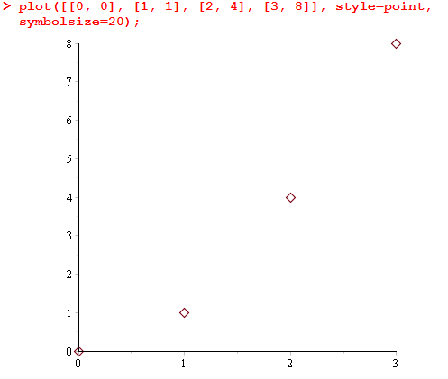
A typical use of [] is to create point plots. To do this, we represent a data point by the ordered pair [x-coordinate, y-coordinate]. Then, we pass plot a list of points, i.e. a nested list. The following example creates a plot of four data points:

> plot([[0, 0], [1, 1], [2, 4], [3, 8]], style=point, symbolsize=20);

Here’s what it should look like when you execute that line; the two style options are just included to make the points easier to see.

While this is cool, it would be great to be able to make a point plot without writing down the whole list explicitly, when the points follow a regular pattern. This can be done by using seq. For example, if we wanted to plot \(\sin(x/2)\) at all integer points from 0 to 30, we’d use the command

> plot([seq([i, sin(i/2)], i=0..30)], style=point, symbolsize=20);

It is very instructive to look closely at exactly how seq was used. The expression being repeated over and over by seq is [i, sin(i/2)], as i goes from 0 to 30. So this creates a list of data points. Immediately surrounding the call to seq there is another pair of [brackets], which dumps all of these points into a list, and this list is what is plotted. We could write equivalently using more lines:

> seqOfPoints := seq([i, sin(i/2)], i=0..30);
> listOfPoints := [seqOfPoints];
> plot(listOfPoints, style=point, symbolsize=20);

Note: you can also see ?plot/parametric for another way of doing parametric plots like the above.

For the next exercise, which will be the last item in this lesson, we need a way to count the number of elements in a set. The nops() function accomplishes this:

> nops({1, 2, 1, 3, 10, 9, 2});
# gives back 5, the number of elements in {1, 2, 3, 9, 10}