M-6: Creating Procedures

We already saw how to create a new mathematical function using the -> operator. This lesson focuses on Maple procedures. (In general, for programming, there is not a strong distinction between functions and procedures so be aware that we occasionally use different words for the same thing.)

A procedure is a set of rules for taking some input, doing some steps, and then giving back (returning) an output. The new generality beyond ->-style functions comes from the fact that we will be able to declare multiple instructions as part of the procedure definition.

Here’s a tiny example of a procedure that returns the square of its input:

> square := proc(x);
     return x*x;
  end;

As you might guess, after executing this line, square(5) will give back 25 and square(y^2) will give back y⁴. Try this yourself and be careful to use the shift-enter method introduced in the previous lesson.

The general form of a procedure definition is

> «procedure name» := proc(«sequence of arguments»);
     «body»
  end;

where there can be 0, 1, 2, or any number of arguments. Arguments means the same as inputs for a procedure. (If you’re skeptical that any useful procedure could have 0 arguments, try running rand(). Other situations are when you want to interact with user input or output, access the printer or files, or if the procedure has some side effects on global variables.)

return of the proc

Wherever the statement

return «value»

is found inside of your procedure body, the procedure immediately quits and gives back the stated value to whatever called the procedure. So the following code is another way of finding the absolute value:

> absValue := proc(x);
     if x < 0 then
        return -x;   # 1st return statement
     end:
     return x;       # 2nd return statement
  end;

You don’t have to use an else clause because the procedure could only possibly get to the 2nd return statement if the body of the if statement (the 1st return) is not evaluated.

Maple will allow you to leave out the return statement if it’s on the last line, but we strongly recommend using explicit returns like above to keep your style consistent, readable, and error-free. (A common cause of errors is forgetting to return. For example, what happens to the procedure above if we change the 3rd line to just -x;?)

Local Variables

Sometimes you’ll want to write a complicated procedure that has some intermediate steps. As we have done many times before, we’ll use the quadratic equation as an example. Let’s create a procedure that takes inputs (arguments) a, b, and c and returns the set of all real zeroes to \(ax^2+bx+c=0\). We know that computing the discriminant is an important intermediate step and so it makes sense to compute that separately. This gives

> quadraticRootSet := proc(a, b, c);
     disc := b*b-4*a*c;
     if (disc < 0) then
       return {};
     end;
     #... more stuff, square roots, etc   
  end;

By the time we finish writing out this procedure, Maple will warn us that disc is “implicitly declared local.” Accordingly, we will explicitly declare it as local to make the warning go away:

> quadraticRootSet := proc(a, b, c) local disc;
  #... as before

That is to say: immediately after the argument list and before any (semi)colon, type local and then the sequence of all variables you want to declare as local variables for that procedure.

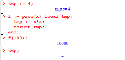
Maple complains about this because you could in principle also want to declare disc as global. (See ?global for details.) The point of a local variable is that it does not interfere with any other variables defined with the same name in other places. Consider the following set of commands:

We define tmp to equal 4, and even though the procedure f also sets tmp to 10000, this is a different variable of the same name. So at the end, the tmp that we print still has the value of 4. Imagine a long Maple document with a dozen inter-related procedures, each with a loop counter variable i, and you can begin to appreciate why it makes sense to give each procedure its own local scope (a.k.a. local namespace).

Memoization

Often, a procedure should have its output depending solely on its arguments. (Functions in the sense of a mathematical relation whose inverse is injective are like this; rand() is an example of one that is not.) In such a case, you can save a great deal of computational effort by remembering past input-output pairs. A typical example is the Fibonacci function:

> fibonacci := proc(n):
     if (n <= 2) then return 1; end:
     return fibonacci(n-1) + fibonacci(n-2);
  end:

Try this and see that it gives the correct first few values. (E.g., run seq(fibonacci(i), i=1..10);)

Now, try to compute fibonacci(25) or fibonacci(30). There will be a noticeable delay in evaluating it! This is surprising, since you will see that these numbers are not so big, and only require doing about thirty additions — or do they?

In fact, you’ve asked Maple to compute the Fibonacci numbers in quite a different way than what you would do by hand. By hand, you’d probably make a list starting from the first few values and adding two each time to get the next one. But you’re telling Maple (we’ll use F for short),

the way to compute F(k) is to call F(k-1) and then call F(k-2) and then add these numbers up.

Now think about what this means for F(30): it requires calling F(29) and F(28). In turn, we’ll eventually have to call F(28) and F(27) once for F(29), and F(27) and F(26) in order to compute F(28). (You can visualize all of the calls as a binary tree.) There is a great deal of redundancy going on and in fact computing F(k) in this way takes F(k) steps; and 0.8 million steps takes a long time, even for Maple.

There are two general techniques called dynamic programming and memoization which can help ameliorate this kind of problem. We’ll only discuss memoization since it has an easy catch-all implementation in Maple; the Sieve of Eratosthenes for computing primes is an example of dynamic programming that you may already know, and the “write down 1, 1, 1+1=2, 1+2=3, …” method for the Fibonacci numbers is another example.

Back to memoization. To apply memoization to a procedure means that

1. we attach a hidden lookup table to the procedure, mapping inputs to outputs
2. when the procedure is called on an input that has not been seen before, we run the procedure body but just before returning, we store the input and output in the table
3. when the procedure is called on an input that has been seen before, we skip the procedure body and just give the value in the table.

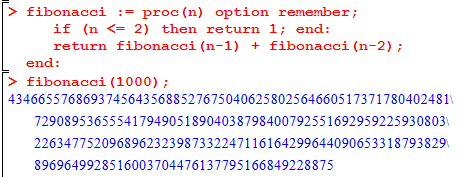
Maple will take care of all of this for you! Add option remember; after the variable list (before or after the local variables, if they are present).

This runs much faster: computing F(k) with memoization uses fewer than 2k calls, much less than the F(k) ~ \(1.6^k\) many calls used by the non-memoized version.

Procedures versus Functions

As a final note, there are some things that are easy to do with ->-style functions which are not so easy with procedures. To give just one example, suppose we want to find the roots of a procedure such as absValue above. The solve procedure is unable to cope with this setting, and so is its floating-point cousin fsolve. Although it is beyond the scope of this course, you would probably want to use the bisection method (binary search) in this setting.