3-5: Graphics

In this lesson we’ll discuss several ways of creating graphics for your LaTeX document.

• Inkscape and IPE are two graphical “what-you-see-is-what-you-get” programs. They allow you to create images that have LaTeX text embedded in them (for example, a label like $y=|x-2|$) and then generate LaTeX documents including these images.
  • They have slightly different workflows, as described below.
• It’s not for the faint of heart, but if you like programming, you may enjoy the flexibility and precision gained from programmatic graphics, where the diagram is specified via commands. In this lesson we give brief examples of the pstricks package for drawing 2D (or 3D) graphics and the pgfplots package for making line and bar charts.

GeoGebra can export to pstricks, and with Maple you can create arbitrary data that you can feed into pgfplots. So keep these packages in mind for Assignment 6, in which one requirement is that you integrate two of the tools discussed in the course.

Using LaTeX in Graphics Editors

Here are very short explanations of how to use IPE and Inkscape. The methods are quite different and the programs themselves have very different interfaces, but the final results are very similar, so which one you prefer may be a matter of taste.

Both are “vector” graphics editors.  This means they can be used to make drawings which can be stretched or shrunk without losing information or becoming pixelated (LaTeX documents are vector graphics as well).

In both cases: the way to get LaTeX math text to show up is to create a text object in the editor. By default, these will be rendered in text mode, but like in LaTeX, anything in-between dollar signs will be interpreted in math, so for example writing point $x_4$ as the text will result in \(\textrm{point }x_4\) appearing in the final result. The instructions below assume you’ve already drawn some things and added some text in this way.

Disclaimers:

1. the instructions below might be slightly different depending on your operating system, since it’s only been tested on Windows 7.
2. Inkscape and IPE are separate programs that you have to install. The homepages, where you can obtain the installer files and documentation, are here for Inkscape and here for IPE.

IPE

• Inside of the editor, to render the dollar signs as LaTeX math, choose Run LaTeX from the File menu.
• To use the diagram in your documents, click Save as, and choose PDF for the file type.
• Use \includegraphics to include the PDF as we described last week.

Inkscape

• Inside of Inkscape, draw some images, then create text boxes and use dollar signs that contain LaTeX math.
  • Inside of Inkscape, it will just look like dollar signs.
• Click Save As… and select PDF format.
• You’ll see a pop-up window with some options: you must check the box “PDF+LaTeX” option. Then save (press OK). It will create two files, one ending in .pdf and the other in .pdf_tex: it’s important that you don’t rename them, although it’s fine to move them to a different directory. They should be in the same directory as your .tex file. You should have no need to open or edit the .pdf_tex file, instead you will feed to the \input command (below).

In your main .tex document:

• Include the packages \usepackage{color, graphicx} in your preamble
• Where you would normally use the includegraphics command, instead put the following:

\def\svgwidth{\columnwidth}
\input{«filenameYouChose».pdf_tex}

• When you compile (you may need to use xelatex for this if your normal compiler doesn’t work, see below).
• You can resize the image and/or use it as a float. See here for more info.

pgfplots

The pgfplots package is used to create line/bar graphs, such as this one:

It’s true that you can use Excel, Google Documents, or other programs to create charts and then include them as graphics in .png/.pdf format. What are the pros of using pgfplots?

• The diagram font will exactly match the paper font and its size, avoiding weird scaling issues or tiny labels
• You can put LaTeX math symbols in the labels, legends and captions
• When you want to change a data point or how the plot is displayed, you don’t need to go back and re-export the file

Let’s get to the actual instructions. In order to produce the chart above, we used the following text:

\documentclass{article}
\usepackage{pgfplots}
\begin{document}
% VV remove if you don't want a float VV
\begin{figure} 
\centering 
% ^^ end optional float part ^^
\begin{tikzpicture}
\begin{axis}[xlabel=Month,ylabel=\# days in month]
\addplot coordinates {
(1, 31) (2, 28.2425) (3, 31)
(4, 30) (5, 31) (6, 30)
(7, 31) (8, 31) (9, 30)
(10, 31) (11, 30) (12, 31)
};
\end{axis}
\end{tikzpicture}
% VV remove if you don't want a float VV
\caption{The number of days in each month of the year.}
\end{figure}
% ^^ end optional float part ^^
\end{document}

Read the source code, which should be fairly self-explanatory, and can serve as a template for you to get started. There are a lot of options in pgfplots, but let’s talk about two that might be useful here. Suppose we think that the display of the diagram is bad: we want the y-axis to start at 0, and we want it to look like a bar graph. To fix this, add the two options  ybar,ymin=0 to the existing axis options (e.g., before xlabel). Try this out and see what you get.

You can do a lot of other things with this package: create semi-log or log-log plots by replacing the axis environment with another one; change where the axis lines show up; reduce extra space with the option enlargelimits=false; change the labels or the appearance of ticks and grids; customize the labels; and put multiple plots on one graph. Here is an example:

The source code for this diagram has two parts, the .tex part and the data file. We encourage you to try searching the extensive documentation, which has lots of examples, to learn more about how to use pgfplots. You can also find many samples online, e.g. here.

pstricks

The pstricks package is an extremely sophisticated programmatic graphic creation package for LaTeX. It can create plots, geometric diagrams, graph theory pictures, and much more. Check out the official pstricks “gallery” here.

This package gives you precise control of whether your diagram’s vertices are in the right spots, and for complex diagrams, lets you use loops and subcommands. However, if you choose to use pstricks for your final project, do not feel the need that you have to become an expert; it is enough that you find useful portions of it that you understand, and that you use it to communicate graphically in an effective way.

(pstricks gets its name from the PostScript language. It was for many years the most common output format of LaTeX. It still is in a sense, because it is a component of the PDF format.)

Here is an example of drawing a picture with pstricks:

\documentclass{article}
\usepackage{pstricks}
\begin{document}
% Boundary will run from (0,0) in the bottom left to (5, 5) top right
\begin{pspicture}(5,5) 
   % Triangle in red:
   \psline[linecolor=red](1,1)(5,1)(1,4)(1,1)
   % Bezier curve in green:
   \pscurve[linecolor=green,linewidth=2pt,%
     showpoints=true](5,5)(3,2)(4,4)(2,3)
   % Circle in blue with radius 1:
   \pscircle[linecolor=blue,linestyle=dashed](3,2.5){1}
 \end{pspicture}
\end{document}

This will produce a picture like: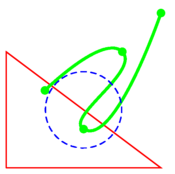

pstricks requires a slightly different compilation system. For both the TeXworks editor and the ShareLaTeX editor, what you need to do is change the compiler to XeLaTeX (rather than the default, pdfLaTeX). This is done using the settings, accessible in the top left. This may be somewhat slower than the pdfLaTeX compiler you were using before.

In case XeLaTeX doesn’t exist on your system, refer to the details in the appendix describing the compiler chain that existed prior to XeLaTeX.

As with pgfplots, the documentation for pstricks is the primary resource; while the package is complex, the documentation is well-written with lots of examples. If you only want to use pstricks with GeoGebra, then you don’t need to read much other than the unit scaling option.

Appendix: PostScript Compiler Chain for pstricks

The below instructions assume you’ve saved the example above to a file, for example \tmp\example.tex.

1. Open a command terminal: on windows press [Windows Key]-R and type cmd; on Mac, go to Terminal via the Spotlight search.
2. Change current directory to where you saved the file:
   cd \tmp
   (on a Mac or Linux, use /tmp instead)
3. latex example.tex
   where example.tex is the filename. This will create example.dvi (or give you error messages)
4. dvips example.dvi
   which will create example.ps
5. ps2pdf example.ps
   which will finally create example.pdf
6. View the pdf. On most systems a shortcut is just typing example.pdf at the command prompt.

If you’re continuing to edit the file, repeat steps 3-6 as you work on it.